Welcome to
TheRecallProblem.com
Three staffing industry articles (below)
explaining the collapse of the industry.
Those agencies that provide the
best customer service will survive.
Read more below.
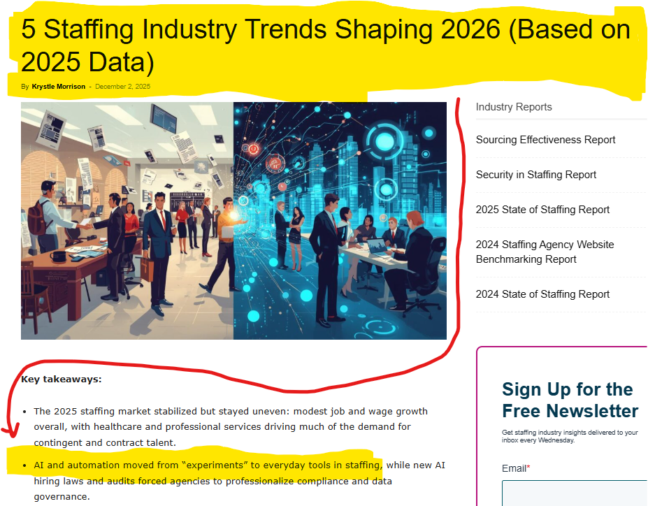
Article #1:
AI is killing the industry.
(from the article: Link to article below)
"AI and automation moved from experiments to everyday tools in staffing, while new AI hiring laws and audits forced agencies to professionalize compliance and data governance."
Click here to read it yourself
Article #2:
More bad news for the staffing industry.
The industry is at a 14 year low.
(from the article: Link to article below)
1.
In the wake of its historic peak, the US staffing industry has experienced a decline for 23 of the past 24 months. In the first quarter of 2024 alone, the staffing industry lost 186,000 jobs, a decline of 7.7% from 4Q23 to 1Q24.
2.
However, in an unsettling reverse of trends, the number of temporary workers supplied via staffing agencies has steadily declined since June 2022 (over 4 years of decline)
3.
As of May 2024, (staffing agency) employment dropped by 6.5% from the previous year and 14.2% from its peak in March 2022. (20.7% decline in only two years.)
4.
Excluding the pandemic dip in 2020, the number of temporary help services jobs has not been this low since April 2014, roughly a decade ago.
5.
The current downturn is striking given it follows a decade of US economic expansion (2010-2020) and a pandemic-driven boom (2021-2022).
6.
The 2025 staffing market stabilized but stayed uneven: modest job and wage growth overall, with healthcare and professional services driving much of the demand for contingent and contract talent.
Click here to read it yourself
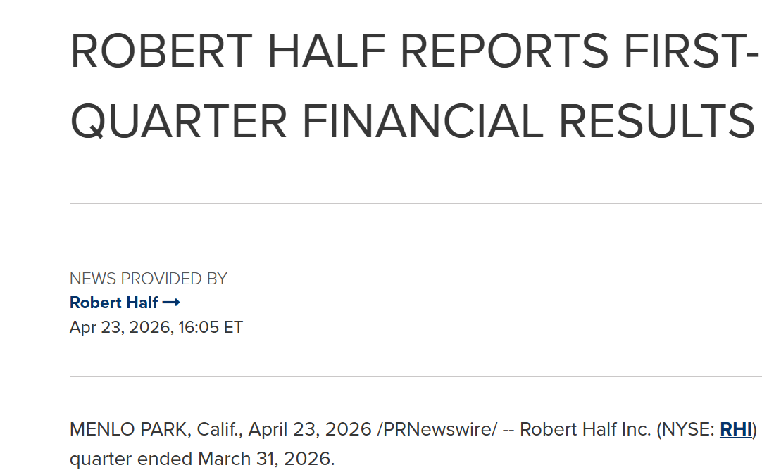
Article #3:
More bad news for the staffing industry
More bad news: Robert Half: Bad News
for Staffing Industry Q1/2026.
March 31, 2026: Industry is collapsing.
ChatGpt summary of the article (below).
Staffing Industry Reality = Revenue is declining year over year
1. $1.300B in Q1 2026 vs $1.352B in Q1 2025 → Down ~4%
2. Profit is shrinking
3. Net income dropped from $17M → $14M
4. Core staffing segments are down
5. Finance & accounting: declining
6. Administrative support: declining
7. Contract talent overall: declining
8. Demand is unstable
9. Slight improvement in some areas
10. But overall trend still negative or uneven
Key Risks
1. AI adoption impacting the industry
2. Increased competition
3. Difficulty attracting talent
4. Margin pressure
5. Economic uncertainty
Bottom Line
The staffing industry is contracting
Revenue, profit, and placements are all under pressure
Even a major player like Robert Half is feeling it.
What this means
The industry isn’t collapsing overnight…
but it is slowly bleeding revenue, margin, and stability
And most agencies:
1. Don’t understand why
2. Don’t see the hidden losses
3. Don’t have a system to fix it
Click here to read it yourself
THE GOOD NEWS?
I HAVE A SYSTEM TO FIX IT.
I can show you how to save your agency.
Half of you will go out of business and the other half will not only survive but thrive.
Those of you that offer the "best in class" admin professionals are the agencies that will thrive.
AI will replace admin professionals last.
YOUR SOLUTION? Read below.
For only $5,000, I will spend a full-day (8 hours) showing you and your staff the 5 steps you must take to allow your agency win the war with AI (artificial intelligence). Training for you and your staff is virtual / online and we can schedule the 8 hours around your availability.
Call me. Let us talk. Talking is free. Let me show you how you are losing your agency. I will prove it to you. Then you can decide if you want to pay me to help you save your agency.
Who am I and why listen to me?
My name is Tim Owens and I have over 25 years experience in the admin industry.
I have owned a training company.
I have hired, tested, and fired admin professionals for multiple clients.
For 25 years I have sat at the desk with admin professionals and observed them work during their day using Microsoft Word and Excel. It is this 25 years of observing that has given me the insight that no one else has.
This insight and knowledge is the knowledge I will share with you to help you save your business from AI and the economy.
The good times and easy money are over for the staffing agency. AI is here. I will show you how to allow your agency to THRIVE while the others go bankrupt.
For 13 years Hilton has relied on me to help their admin professionals work smarter, not harder, with less stress.
Hilton admin professionals love me. IAAP (International Association of Administrative Professionals) love me and more!
Hilton Hotels World-Wide DOES NOT keep an admin professional consultant for 13 years unless HUGE value is brought.
Click the images below to see what they say. I will show you how to save your agency.


Tim Owens
25 years experienced admin professional consultant.
Email:
tvowens@outlook.com
Leave me a message.
310-625-7711
Los Angeles Office / Texting not available
"AI and automation moved from experiments to everyday tools in staffing, while new AI hiring laws and audits forced agencies to professionalize compliance and data governance."
Click here to read it yourself
More bad news for the staffing industry.
The industry is at a 14 year low.
More bad news for the staffing industry
for Staffing Industry Q1/2026.
March 31, 2026: Industry is collapsing.
ChatGpt summary of the article (below).
Staffing Industry Reality = Revenue is declining year over year
1. $1.300B in Q1 2026 vs $1.352B in Q1 2025 → Down ~4%
2. Profit is shrinking
3. Net income dropped from $17M → $14M
4. Core staffing segments are down
5. Finance & accounting: declining
6. Administrative support: declining
7. Contract talent overall: declining
8. Demand is unstable
9. Slight improvement in some areas
10. But overall trend still negative or uneven
Key Risks
1. AI adoption impacting the industry
2. Increased competition
3. Difficulty attracting talent
4. Margin pressure
5. Economic uncertainty
Bottom Line
The staffing industry is contracting
Revenue, profit, and placements are all under pressure
Even a major player like Robert Half is feeling it.
What this means
The industry isn’t collapsing overnight…
but it is slowly bleeding revenue, margin, and stability
And most agencies:
1. Don’t understand why
2. Don’t see the hidden losses
3. Don’t have a system to fix it
Click here to read it yourself
THE GOOD NEWS?
I HAVE A SYSTEM TO FIX IT.
I can show you how to save your agency.
Half of you will go out of business and the other half will not only survive but thrive.
25 years experienced admin professional consultant.
tvowens@outlook.com
310-625-7711
Los Angeles Office / Texting not available